3 Background & Historical Context
- Blastic plasmacytoid dendritic cell neoplasm (BPDCN) is an aggressive hematologic malignancy derived from precursors of plasmacytoid dendritic cells (pDCs), listed as a separate entity in the 5th edition of the WHO classification of hematolymphoid tumors.
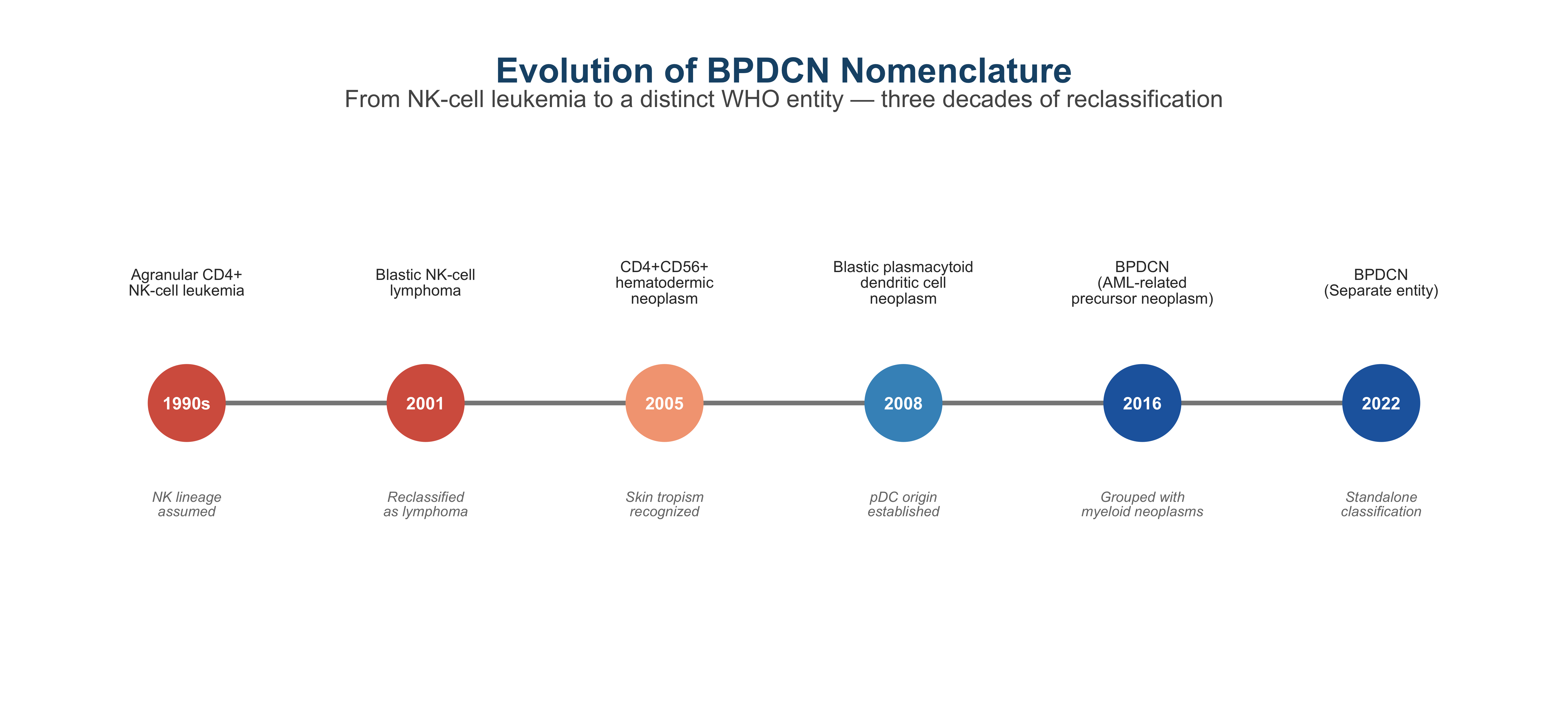
- The disease has undergone a series of name and classification changes over decades — previously termed CD4⁺CD56⁺ hematodermic neoplasm, blastic NK-cell lymphoma, and agranular CD4⁺ natural killer cell leukemia — reflecting historical confusion before its true pDC lineage was established.
- BPDCN constitutes approximately 0.44% of all hematologic malignancies (~0.05 cases per 100,000), but this likely represents an underestimation due to heterogeneous presentation and diagnostic challenges.
- The approval of tagraxofusp (2018) and ongoing development of pivekimab sunirine have made accurate diagnosis imperative, as CD123-directed therapies require precise identification of this entity.
3.1 Historical Nomenclature
Show code
library(ggplot2)

nomenclature <- data.frame(
  era = factor(c(
    "1990s",
    "2001",
    "2005",
    "2008\n(WHO 4th Ed.)",
    "2016\n(WHO Revised)",
    "2022\n(WHO 5th Ed.)"
  ), levels = c(
    "1990s",
    "2001",
    "2005",
    "2008\n(WHO 4th Ed.)",
    "2016\n(WHO Revised)",
    "2022\n(WHO 5th Ed.)"
  )),
  name = c(
    "Agranular CD4+\nNK-cell leukemia",
    "Blastic NK-cell\nlymphoma",
    "CD4+CD56+\nhematodermic\nneoplasm",
    "Blastic plasmacytoid\ndendritic cell\nneoplasm",
    "BPDCN\n(AML-related\nprecursor neoplasm)",
    "BPDCN\n(Separate entity)"
  ),
  y = rep(1, 6),
  insight = c(
    "NK lineage\nassumed",
    "Reclassified\nas lymphoma",
    "Skin tropism\nrecognized",
    "pDC origin\nestablished",
    "Grouped with\nmyeloid neoplasms",
    "Standalone\nclassification"
  )
)

color_gradient <- c("#d6604d", "#d6604d", "#f4a582", "#4393c3", "#2166ac", "#2166ac")

ggplot(nomenclature, aes(x = era, y = y)) +
  geom_segment(
    data = data.frame(
      x = levels(nomenclature$era)[1:5],
      xend = levels(nomenclature$era)[2:6],
      y = 1, yend = 1
    ),
    aes(x = x, xend = xend, y = y, yend = yend),
    inherit.aes = FALSE,
    arrow = arrow(length = unit(0.2, "cm"), type = "closed"),
    color = "#888888", linewidth = 1
  ) +
  geom_point(size = 16, color = color_gradient) +
  geom_text(aes(label = gsub("\\n.*", "", as.character(era))),
            size = 2.8, fontface = "bold", color = "white") +
  geom_text(aes(label = name, y = y + 0.18), size = 2.5, color = "#333333",
            lineheight = 0.85) +
  geom_text(aes(label = insight, y = y - 0.15), size = 2.3, color = "#777777",
            fontface = "italic", lineheight = 0.85) +
  scale_y_continuous(limits = c(0.65, 1.35)) +
  labs(
    title = "Evolution of BPDCN Nomenclature",
    subtitle = "From NK-cell leukemia to a distinct WHO entity — three decades of reclassification"
  ) +
  theme_void(base_size = 13) +
  theme(
    plot.title = element_text(hjust = 0.5, face = "bold", size = 16, color = "#1a5276"),
    plot.subtitle = element_text(hjust = 0.5, size = 11, color = "#555555",
                                 margin = margin(b = 15)),
    plot.margin = margin(20, 20, 20, 20)
  )
4 Clinical Presentation
4.1 Demographics
Show code
library(ggplot2)
library(dplyr)
library(tidyr)

demo_data <- tibble(
  Characteristic = c(
    "Median age ≥65 years",
    "Male sex",
    "White race",
    "ECOG PS 0",
    "ECOG PS 1",
    "Skin involvement",
    "Bone marrow",
    "Lymph nodes",
    "Peripheral blood",
    "CNS (occult or overt)"
  ),
  `Tagraxofusp\nPivotal (n=47)` = c(83, 81, 91, 47, 53, 94, 51, 45, 17, 12),
  `PVEK CADENZA\n(N=84)` = c(71, 82, 82, 36, 61, 77, 48, 36, 16, 8),
  `French BPDCN\nNetwork` = c(73, 77, 88, NA, NA, 84, 51, 45, 45, 15)
)

demo_long <- demo_data |>
  pivot_longer(-Characteristic, names_to = "Cohort", values_to = "Percentage") |>
  filter(!is.na(Percentage)) |>
  mutate(
    Characteristic = factor(Characteristic, levels = rev(demo_data$Characteristic)),
    Cohort = factor(Cohort, levels = c(
      "Tagraxofusp\nPivotal (n=47)",
      "PVEK CADENZA\n(N=84)",
      "French BPDCN\nNetwork"
    ))
  )

cohort_colors <- c(
  "Tagraxofusp\nPivotal (n=47)" = "#2166ac",
  "PVEK CADENZA\n(N=84)" = "#d6604d",
  "French BPDCN\nNetwork" = "#4daf4a"
)

ggplot(demo_long, aes(x = Percentage, y = Characteristic, fill = Cohort)) +
  geom_col(position = position_dodge(width = 0.8), width = 0.7, alpha = 0.9) +
  geom_text(
    aes(label = paste0(Percentage, "%")),
    position = position_dodge(width = 0.8),
    hjust = -0.15, size = 2.8, fontface = "bold"
  ) +
  scale_fill_manual(values = cohort_colors) +
  scale_x_continuous(
    limits = c(0, 110),
    breaks = seq(0, 100, 25),
    labels = function(x) paste0(x, "%")
  ) +
  labs(
    title = "Baseline Patient Characteristics at BPDCN Diagnosis",
    subtitle = "Cross-study comparison of demographic and disease involvement patterns",
    x = "Patients (%)",
    y = NULL,
    fill = "Study Cohort"
  ) +
  theme_minimal(base_size = 13) +
  theme(
    plot.title = element_text(face = "bold", size = 16, color = "#1a5276"),
    plot.subtitle = element_text(size = 12, color = "#555555", margin = margin(b = 15)),
    legend.position = "bottom",
    legend.title = element_text(face = "bold"),
    panel.grid.major.y = element_blank(),
    panel.grid.minor = element_blank(),
    axis.text.y = element_text(size = 11),
    plot.margin = margin(15, 30, 15, 15)
  )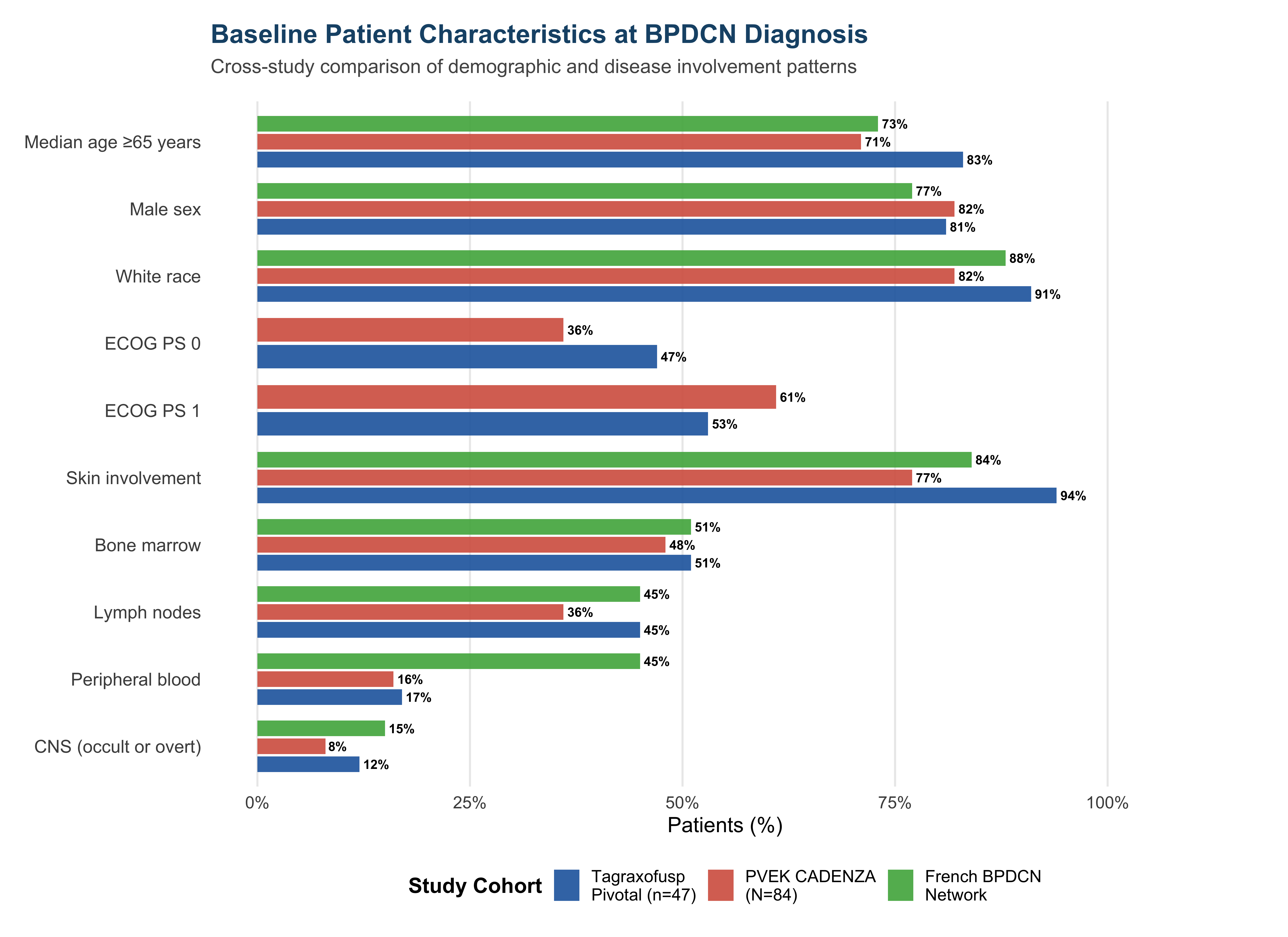
Skin involvement occurs in 65–94% of patients and is the most common presenting feature. Characteristic lesions include dark purple or violaceous nodules, plaques, and tumors — often initially in sun-exposed areas. BPDCN has been misdiagnosed as melanoma, leprosy, and even dermatomyositis. Importantly, tumor phylogenomics shows that premalignant clones in the bone marrow give rise to skin tumors, highlighting that even seemingly “localized” skin disease is a systemic malignancy.
4.2 Disease Compartments at Diagnosis
Show code
import matplotlib.pyplot as plt
import numpy as np

compartments = ['Skin', 'Bone Marrow', 'Lymph Nodes', 'Peripheral Blood', 'CNS', 'Viscera']
percentages = [84, 51, 45, 45, 15, 14]

fig, ax = plt.subplots(figsize=(10, 5.5))

colors = ['#2166ac', '#4393c3', '#67a9cf', '#92c5de', '#d1e5f0', '#e0e0e0']

bars = ax.barh(
    range(len(compartments)), percentages,
    color=colors, edgecolor='white', linewidth=1.5, height=0.6
)

for bar, pct in zip(bars, percentages):
    ax.text(
        bar.get_width() + 1.5, bar.get_y() + bar.get_height()/2,
        f'{pct}%', va='center', ha='left', fontsize=13, fontweight='bold',
        color='#333333'
    )

ax.set_yticks(range(len(compartments)))
ax.set_yticklabels(compartments, fontsize=12, fontweight='bold')
ax.set_xlim(0, 100)
(0.0, 100.0)Show code
ax.set_xlabel('Patients (%)', fontsize=12)
ax.set_title(
    'BPDCN Disease Compartments at Diagnosis',
    fontsize=16, fontweight='bold', color='#1a5276', pad=15
)

ax.invert_yaxis()
ax.spines['top'].set_visible(False)
ax.spines['right'].set_visible(False)
ax.spines['left'].set_visible(False)
ax.tick_params(left=False)
ax.grid(axis='x', alpha=0.3, linestyle='--')

fig.text(0.5, -0.02,
         'Data synthesized from French BPDCN Network (Garnache-Ottou et al., Blood Adv 2019) and Kharfan-Dabaja et al., Blood 2025.',
         ha='center', fontsize=8, fontstyle='italic', color='#888888')

plt.tight_layout()
plt.show()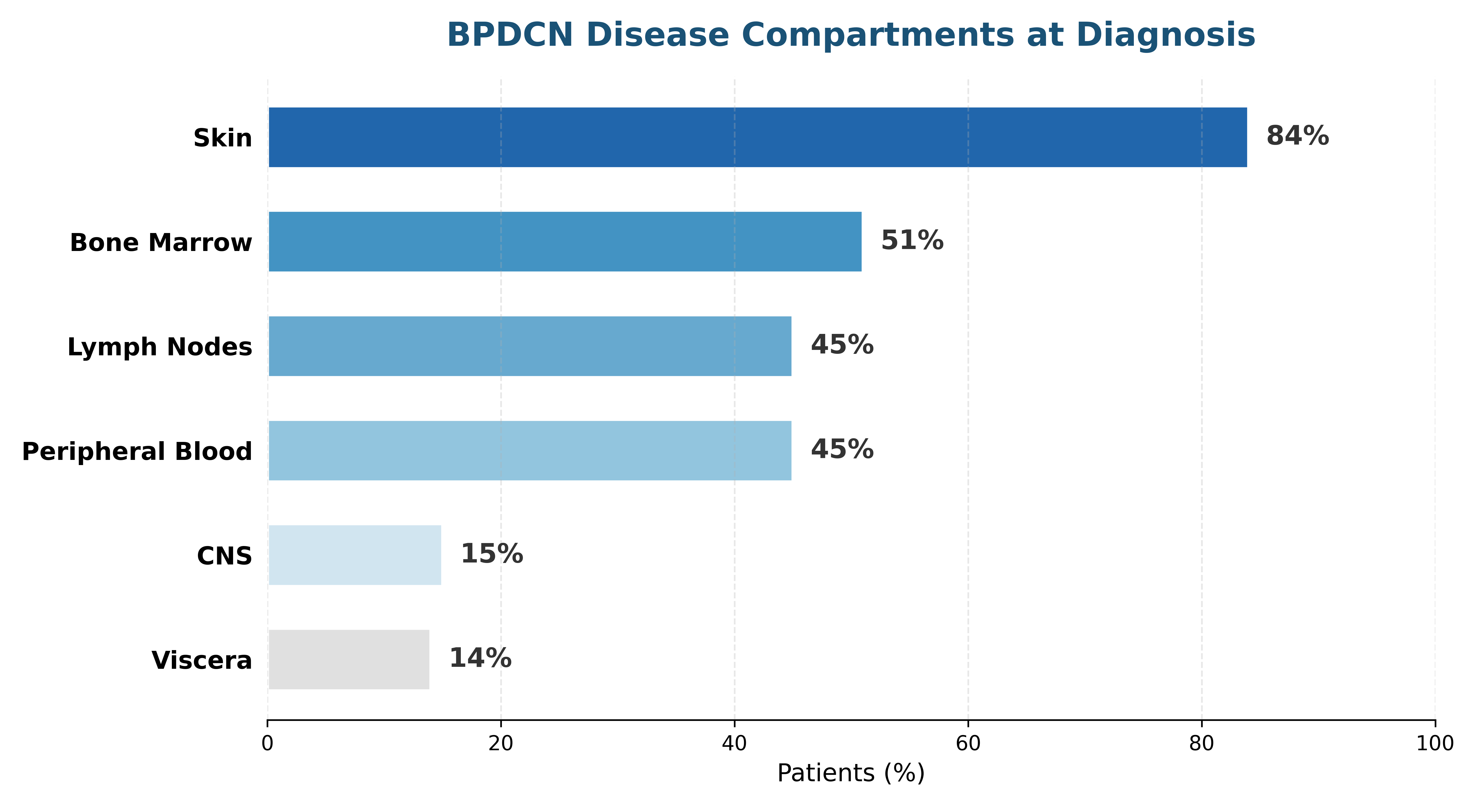
4.3 Hematologic Findings at Diagnosis
Show code
library(ggplot2)

heme_data <- data.frame(
  Finding = factor(c(
    "Blast infiltration\n(bone marrow)",
    "Thrombocytopenia",
    "Anemia",
    "Cytogenetic\nabnormality",
    "Neutropenia",
    "Dysplastic features"
  ), levels = c(
    "Blast infiltration\n(bone marrow)",
    "Thrombocytopenia",
    "Anemia",
    "Cytogenetic\nabnormality",
    "Neutropenia",
    "Dysplastic features"
  )),
  Percentage = c(96, 75, 64, 60, 38, 31),
  Category = c("Marrow", "Cytopenias", "Cytopenias", "Genetics", "Cytopenias", "Morphology")
)

cat_colors <- c(
  "Marrow" = "#2166ac",
  "Cytopenias" = "#d6604d",
  "Genetics" = "#4daf4a",
  "Morphology" = "#984ea3"
)

ggplot(heme_data, aes(x = Finding, y = Percentage, fill = Category)) +
  geom_col(width = 0.6, alpha = 0.9) +
  geom_text(aes(label = paste0(Percentage, "%")),
            vjust = -0.5, fontface = "bold", size = 5, color = "#333333") +
  scale_fill_manual(values = cat_colors, name = "Category") +
  scale_y_continuous(limits = c(0, 110), breaks = seq(0, 100, 25),
                     labels = function(x) paste0(x, "%")) +
  labs(
    title = "Hematologic Findings at BPDCN Diagnosis",
    subtitle = "French BPDCN Network — Peripheral blood and bone marrow abnormalities",
    x = NULL,
    y = "Patients (%)"
  ) +
  theme_minimal(base_size = 14) +
  theme(
    plot.title = element_text(face = "bold", size = 16, color = "#1a5276"),
    plot.subtitle = element_text(size = 11, color = "#555555", margin = margin(b = 15)),
    legend.position = "bottom",
    legend.title = element_text(face = "bold"),
    panel.grid.major.x = element_blank(),
    panel.grid.minor = element_blank(),
    axis.text.x = element_text(size = 10, face = "bold"),
    plot.margin = margin(15, 20, 15, 15)
  )
5 Immunophenotypic Diagnosis
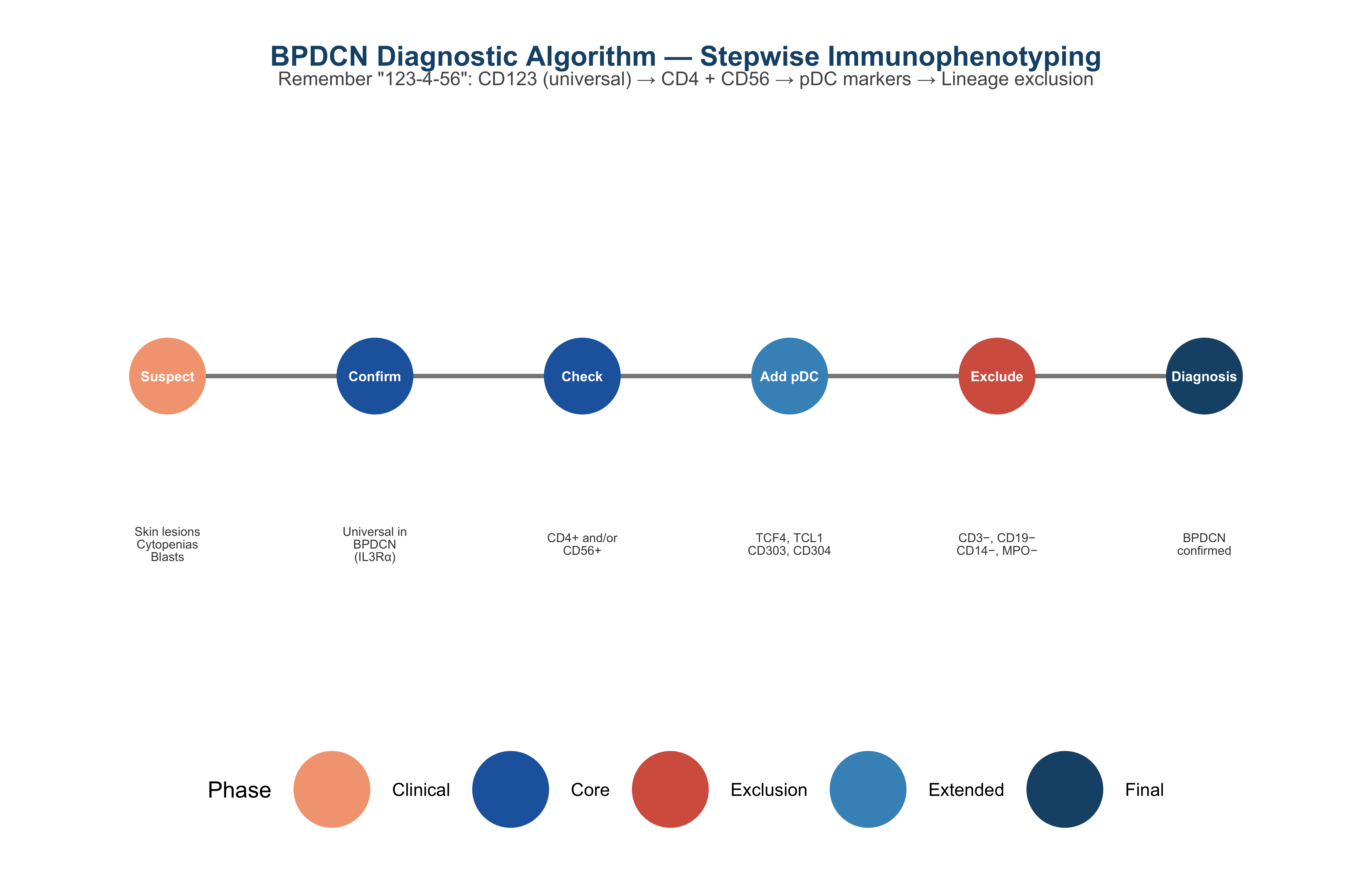
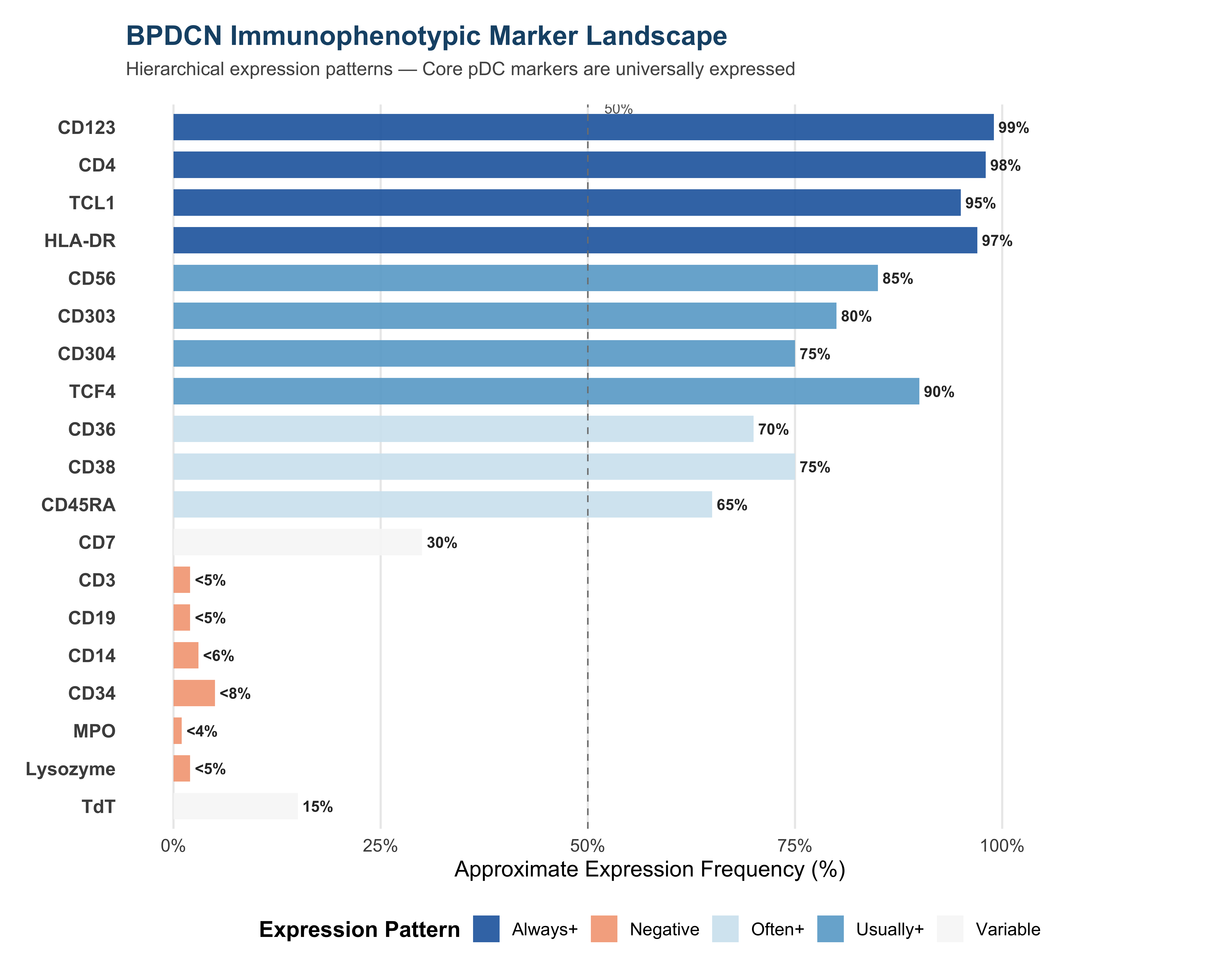
The cornerstone of BPDCN diagnosis is its distinctive immunophenotype. Two complementary diagnostic frameworks are currently in use: the WHO 5th Edition criteria and the NCCN guidelines (v3.2024).
| Criterion | Markers | Requirement |
|---|---|---|
| Pathway A | CD123 + CD4 and/or CD56 + ≥1 pDC marker | Expression of CD123, CD4/CD56, and ≥1 of: TCF4, TCL1, CD303, CD304 |
| Pathway B | ≥3 pDC markers without lineage markers | Any 3 of: CD123, TCF4, TCL1, CD303, CD304 — AND absence of CD3, CD14, CD19, CD34 |
| Expected negative | Lineage exclusion markers | CD3 (T-cell), CD19 (B-cell), CD14 (monocytic), lysozyme, myeloperoxidase |
| Criterion | Markers | Requirement |
|---|---|---|
| Positive markers | ≥4 of 6 BPDCN antigens | CD4, CD56, CD123, TCL1, CD2AP, CD303/BDCA-2 |
| Negative markers | Myeloid lineage exclusion | MPO, lysozyme, CD14, CD34, CD116, CD163 |
| Negative markers | Lymphoid lineage exclusion | T-cell and B-cell markers |
| Marker | Expression | Level |
|---|---|---|
| CD4 | Always expressed | High |
| CD123 | Always expressed | High |
| HLA-DR | Always expressed | High |
| TCL1 | Always expressed | High |
| CD56 | Very often expressed | Variable |
| CD303/BDCA-2 | Very often expressed | Variable |
| CD304 | Very often expressed | Variable |
| CD36, CD38, CD45RA | Very often expressed | Variable |
5.1 Immunophenotypic Diagnostic Algorithm
Show code
library(ggplot2)

steps <- data.frame(
  step = factor(c(
    "1. Suspect\nBPDCN",
    "2. Confirm\nCD123+",
    "3. Check\nCD4/CD56",
    "4. Add pDC\nMarkers",
    "5. Exclude\nLineage",
    "6. Diagnosis\nConfirmed"
  ), levels = c(
    "1. Suspect\nBPDCN",
    "2. Confirm\nCD123+",
    "3. Check\nCD4/CD56",
    "4. Add pDC\nMarkers",
    "5. Exclude\nLineage",
    "6. Diagnosis\nConfirmed"
  )),
  y = rep(1, 6),
  phase = c("Clinical", "Core", "Core", "Extended", "Exclusion", "Final"),
  detail = c(
    "Skin lesions\nCytopenias\nBlasts",
    "Universal in\nBPDCN\n(IL3Rα)",
    "CD4+ and/or\nCD56+",
    "TCF4, TCL1\nCD303, CD304",
    "CD3−, CD19−\nCD14−, MPO−",
    "BPDCN\nconfirmed"
  )
)

phase_colors <- c(
  "Clinical" = "#f4a582",
  "Core" = "#2166ac",
  "Extended" = "#4393c3",
  "Exclusion" = "#d6604d",
  "Final" = "#1a5276"
)

ggplot(steps, aes(x = step, y = y)) +
    geom_segment(
    data = data.frame(
      x = levels(steps$step)[1:5],
      xend = levels(steps$step)[2:6],
      y = 1, yend = 1
    ),
    aes(x = x, xend = xend, y = y, yend = yend),
    inherit.aes = FALSE,
    arrow = arrow(length = unit(0.3, "cm"), type = "closed"),
    color = "#888888", linewidth = 1.2
  ) +
  geom_point(aes(color = phase), size = 20) +
  geom_text(aes(label = gsub("\\d+\\. ", "", gsub("\n.*", "", as.character(step)))),
            size = 2.8, fontface = "bold", color = "white") +
  geom_text(aes(label = detail, y = y - 0.18),
            size = 2.5, color = "#444444", lineheight = 0.85) +
  scale_color_manual(values = phase_colors, name = "Phase") +
  scale_y_continuous(limits = c(0.65, 1.25)) +
  labs(
    title = "BPDCN Diagnostic Algorithm — Stepwise Immunophenotyping",
    subtitle = "Remember \"123-4-56\": CD123 (universal) → CD4 + CD56 → pDC markers → Lineage exclusion"
  ) +
  theme_void(base_size = 13) +
  theme(
    plot.title = element_text(hjust = 0.5, face = "bold", size = 16, color = "#1a5276"),
    plot.subtitle = element_text(hjust = 0.5, size = 11, color = "#555555",
                                 margin = margin(b = 15)),
    legend.position = "bottom",
    plot.margin = margin(20, 25, 20, 25)
  )
5.2 Marker Expression Landscape
Show code
library(ggplot2)
library(dplyr)
library(tidyr)

markers <- tibble(
  Marker = c(
    "CD123", "CD4", "TCL1", "HLA-DR",
    "CD56", "CD303", "CD304", "TCF4",
    "CD36", "CD38", "CD45RA", "CD7",
    "CD3", "CD19", "CD14", "CD34",
    "MPO", "Lysozyme", "TdT"
  ),
  Category = c(
    rep("Core pDC", 4),
    rep("Extended pDC", 4),
    rep("Often Positive", 3),
    "Variable",
    rep("Expected Negative", 6),
    "Variable"
  ),
  Expression = c(
    99, 98, 95, 97,
    85, 80, 75, 90,
    70, 75, 65, 30,
    2, 2, 3, 5,
    1, 2, 15
  ),
  Status = c(
    rep("Always+", 4),
    rep("Usually+", 4),
    rep("Often+", 3),
    "Variable",
    rep("Negative", 6),
    "Variable"
  )
)

markers <- markers |>
  mutate(Marker = factor(Marker, levels = rev(Marker)))

fill_colors <- c(
  "Always+" = "#2166ac",
  "Usually+" = "#67a9cf",
  "Often+" = "#d1e5f0",
  "Variable" = "#f7f7f7",
  "Negative" = "#f4a582"
)

ggplot(markers, aes(x = Expression, y = Marker, fill = Status)) +
  geom_col(width = 0.7, alpha = 0.9) +
  geom_text(
    aes(label = ifelse(Expression >= 10,
                       paste0(Expression, "%"),
                       paste0("<", Expression + 3, "%"))),
    hjust = -0.15, size = 3.2, fontface = "bold", color = "#333333"
  ) +
  geom_vline(xintercept = 50, linetype = "dashed", color = "grey50", linewidth = 0.4) +
  annotate("text", x = 52, y = 19.5, label = "50%", hjust = 0, size = 3, color = "grey40") +
  scale_fill_manual(values = fill_colors, name = "Expression Pattern") +
  scale_x_continuous(limits = c(0, 115), breaks = seq(0, 100, 25),
                     labels = function(x) paste0(x, "%")) +
  labs(
    title = "BPDCN Immunophenotypic Marker Landscape",
    subtitle = "Hierarchical expression patterns — Core pDC markers are universally expressed",
    x = "Approximate Expression Frequency (%)",
    y = NULL
  ) +
  theme_minimal(base_size = 13) +
  theme(
    plot.title = element_text(face = "bold", size = 16, color = "#1a5276"),
    plot.subtitle = element_text(size = 11, color = "#555555", margin = margin(b = 15)),
    legend.position = "bottom",
    legend.title = element_text(face = "bold"),
    panel.grid.major.y = element_blank(),
    panel.grid.minor = element_blank(),
    axis.text.y = element_text(size = 11, face = "bold"),
    plot.margin = margin(15, 30, 15, 15)
  )
6 Differential Diagnosis
One of the most critical aspects of BPDCN diagnosis is distinguishing it from morphologic mimics — both hematopoietic and non-hematopoietic neoplasms that can present with similar skin involvement or immunophenotypic overlap.
6.1 Differential Diagnosis Table
Show code
import matplotlib.pyplot as plt
import numpy as np

fig, (ax1, ax2) = plt.subplots(1, 2, figsize=(14, 7))

# Panel A: Hematopoietic differentials
heme_entities = [
    'AML with\nleukemia cutis',
    'Mature pDC\nproliferation',
    'T-ALL',
    'B-ALL',
    'NK/T-cell\nlymphoma',
    'ATLL',
    'ALCL'
]
heme_key = [
    'MPO+, CD34+\nCD123 variable',
    'CD34+, CD56−\nMature morphology',
    'CD3+, TdT+\ncytoplasmic CD3',
    'CD19+, CD10+\nTdT+',
    'CD3ε+, CD56+\nEBV+ (EBER)',
    'CD4+, CD25+\nHTLV-1+',
    'CD30+, ALK±\nCD4−'
]

colors_heme = ['#2166ac'] * len(heme_entities)
y_pos = range(len(heme_entities))

for i, (entity, key) in enumerate(zip(heme_entities, heme_key)):
    ax1.barh(i, 1, color='#2166ac', alpha=0.15, height=0.7)
    ax1.text(0.02, i, entity, va='center', ha='left', fontsize=10,
             fontweight='bold', color='#1a5276')
    ax1.text(0.55, i, key, va='center', ha='left', fontsize=9,
             color='#555555', linespacing=1.3)

ax1.set_xlim(0, 1)
(0.0, 1.0)Show code
ax1.set_ylim(-0.5, len(heme_entities) - 0.5)(-0.5, 6.5)Show code
ax1.invert_yaxis()
ax1.set_title('Hematopoietic Neoplasms', fontsize=14, fontweight='bold',
              color='#1a5276', pad=10)
ax1.axis('off')
(np.float64(0.0), np.float64(1.0), np.float64(6.5), np.float64(-0.5))Show code
# Panel B: Non-hematopoietic differentials
non_heme_entities = [
    'Melanoma',
    'Merkel cell\ncarcinoma',
    'Angiosarcoma',
    'Kaposi sarcoma',
    'Dermatomyositis\n(mimicry)'
]
non_heme_key = [
    'S100+, HMB-45+\nMelan-A+',
    'CK20+, CD56+\nNeuroendocrine',
    'CD31+, CD34+\nERG+',
    'HHV-8+\nVascular',
    'Skin rash pattern\nAutoantibodies+'
]

for i, (entity, key) in enumerate(zip(non_heme_entities, non_heme_key)):
    ax2.barh(i, 1, color='#d6604d', alpha=0.15, height=0.7)
    ax2.text(0.02, i, entity, va='center', ha='left', fontsize=10,
             fontweight='bold', color='#8b1a1a')
    ax2.text(0.55, i, key, va='center', ha='left', fontsize=9,
             color='#555555', linespacing=1.3)

ax2.set_xlim(0, 1)
(0.0, 1.0)Show code
ax2.set_ylim(-0.5, len(non_heme_entities) - 0.5)(-0.5, 4.5)Show code
ax2.invert_yaxis()
ax2.set_title('Non-Hematopoietic Neoplasms', fontsize=14, fontweight='bold',
              color='#8b1a1a', pad=10)
ax2.axis('off')
(np.float64(0.0), np.float64(1.0), np.float64(4.5), np.float64(-0.5))Show code
plt.suptitle('Differential Diagnosis of BPDCN — Key Distinguishing Features',
             fontsize=16, fontweight='bold', color='#1a5276', y=1.02)

plt.tight_layout()
plt.show()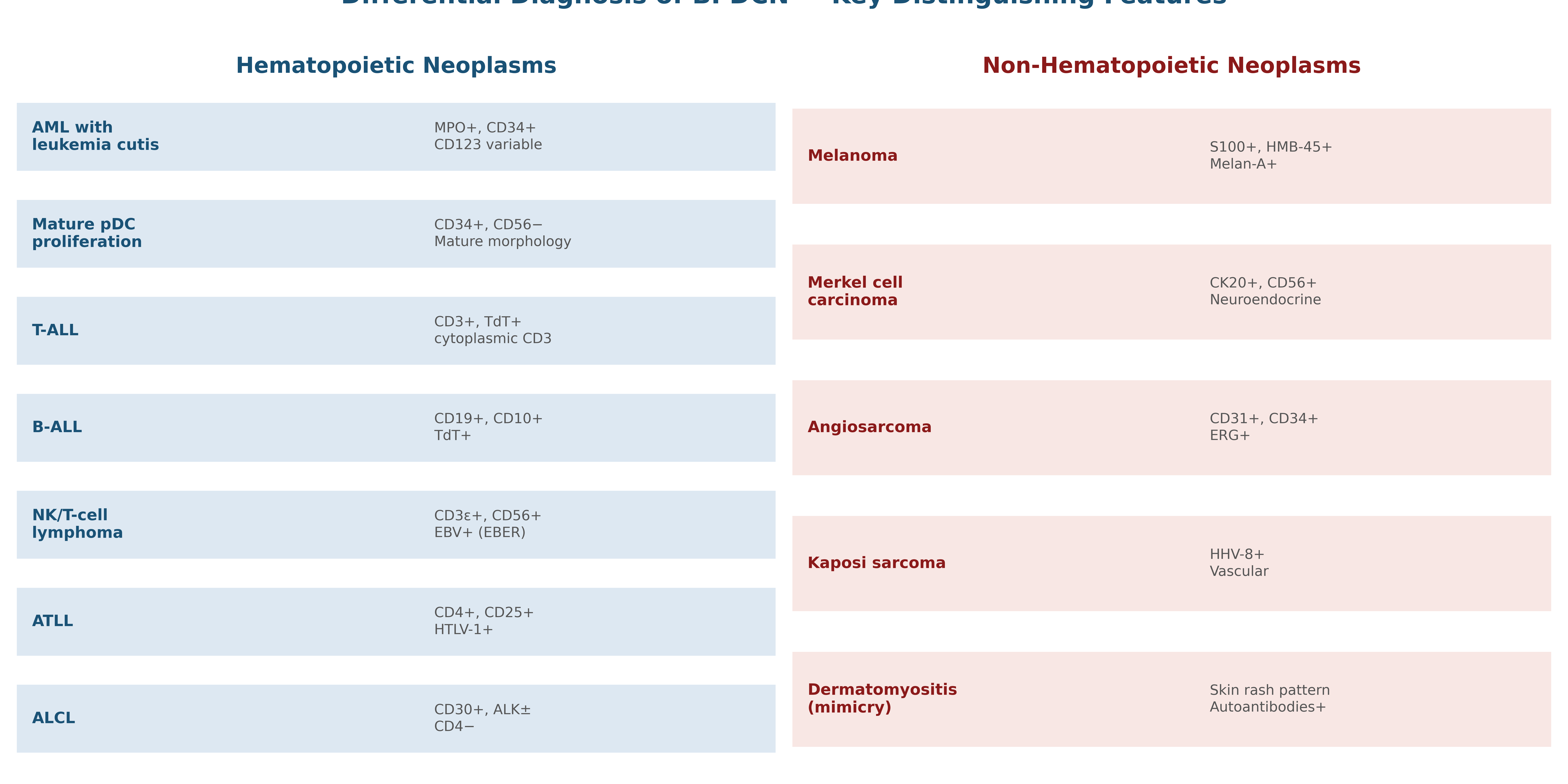
Mature plasmacytoid dendritic cell proliferation — frequently associated with CMML, CML, or AML — must be distinguished from BPDCN. Key differentiators include: mature pDC proliferations are generally CD34-positive and CD56-negative, and cells appear morphologically mature. These proliferations are associated with an underlying myeloid neoplasm and do not warrant BPDCN-directed therapy.
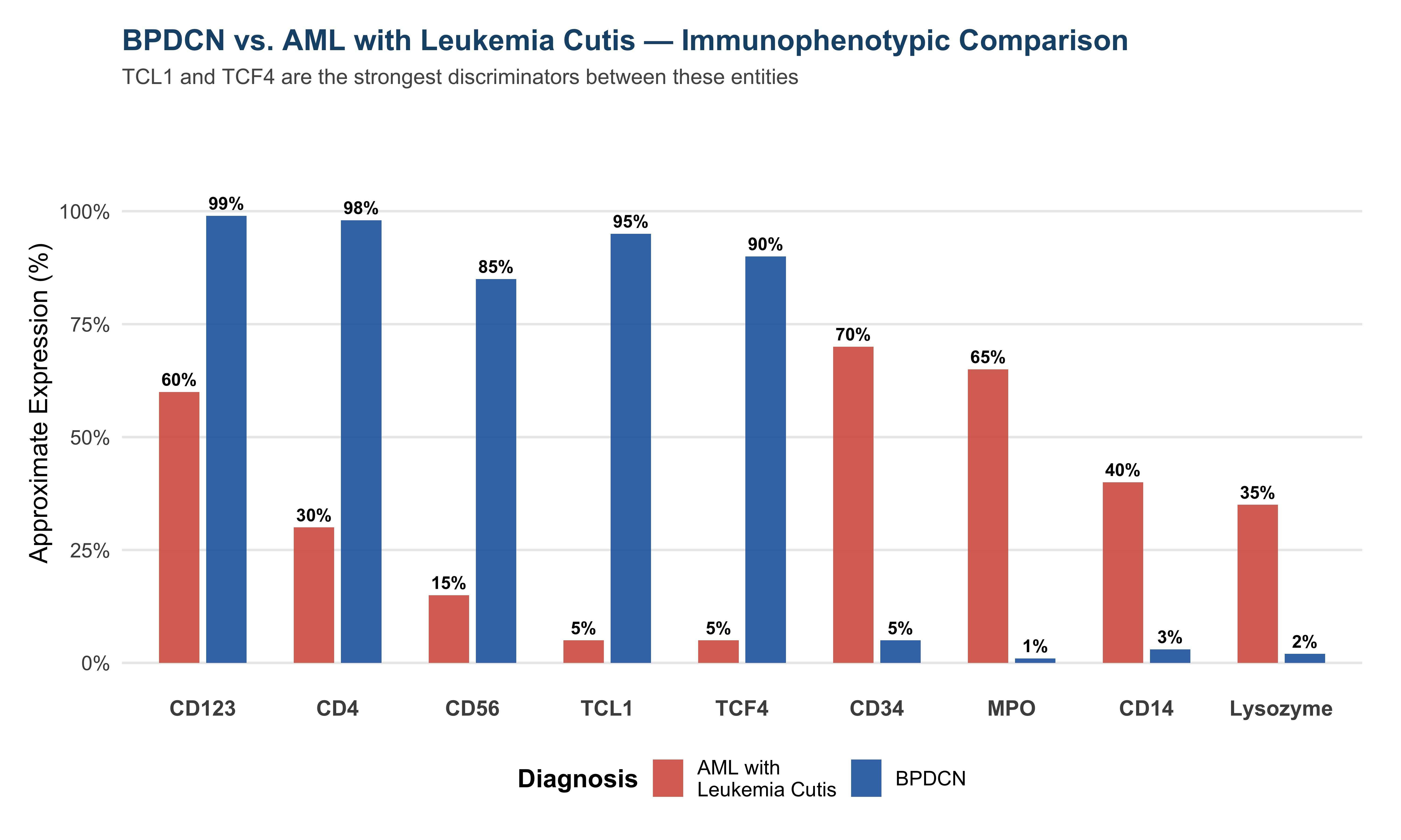
6.2 BPDCN vs. AML with Leukemia Cutis
Show code
library(ggplot2)
library(dplyr)
library(tidyr)

comparison <- tibble(
  Marker = factor(c("CD123", "CD4", "CD56", "TCL1", "TCF4",
                     "CD34", "MPO", "CD14", "Lysozyme"),
                  levels = c("CD123", "CD4", "CD56", "TCL1", "TCF4",
                             "CD34", "MPO", "CD14", "Lysozyme")),
  BPDCN = c(99, 98, 85, 95, 90, 5, 1, 3, 2),
  AML_Cutis = c(60, 30, 15, 5, 5, 70, 65, 40, 35)
)

comp_long <- comparison |>
  pivot_longer(-Marker, names_to = "Disease", values_to = "Expression") |>
  mutate(Disease = ifelse(Disease == "AML_Cutis", "AML with\nLeukemia Cutis", "BPDCN"))

disease_colors <- c("BPDCN" = "#2166ac", "AML with\nLeukemia Cutis" = "#d6604d")

ggplot(comp_long, aes(x = Marker, y = Expression, fill = Disease)) +
  geom_col(position = position_dodge(width = 0.7), width = 0.6, alpha = 0.9) +
  geom_text(
    aes(label = paste0(Expression, "%")),
    position = position_dodge(width = 0.7),
    vjust = -0.5, size = 3.2, fontface = "bold"
  ) +
  scale_fill_manual(values = disease_colors, name = "Diagnosis") +
  scale_y_continuous(limits = c(0, 115), breaks = seq(0, 100, 25),
                     labels = function(x) paste0(x, "%")) +
  labs(
    title = "BPDCN vs. AML with Leukemia Cutis — Immunophenotypic Comparison",
    subtitle = "TCL1 and TCF4 are the strongest discriminators between these entities",
    x = NULL,
    y = "Approximate Expression (%)"
  ) +
  theme_minimal(base_size = 13) +
  theme(
    plot.title = element_text(face = "bold", size = 15, color = "#1a5276"),
    plot.subtitle = element_text(size = 11, color = "#555555", margin = margin(b = 15)),
    legend.position = "bottom",
    legend.title = element_text(face = "bold"),
    panel.grid.major.x = element_blank(),
    panel.grid.minor = element_blank(),
    axis.text.x = element_text(size = 11, face = "bold"),
    plot.margin = margin(15, 20, 15, 15)
  )
7 Genomic Landscape
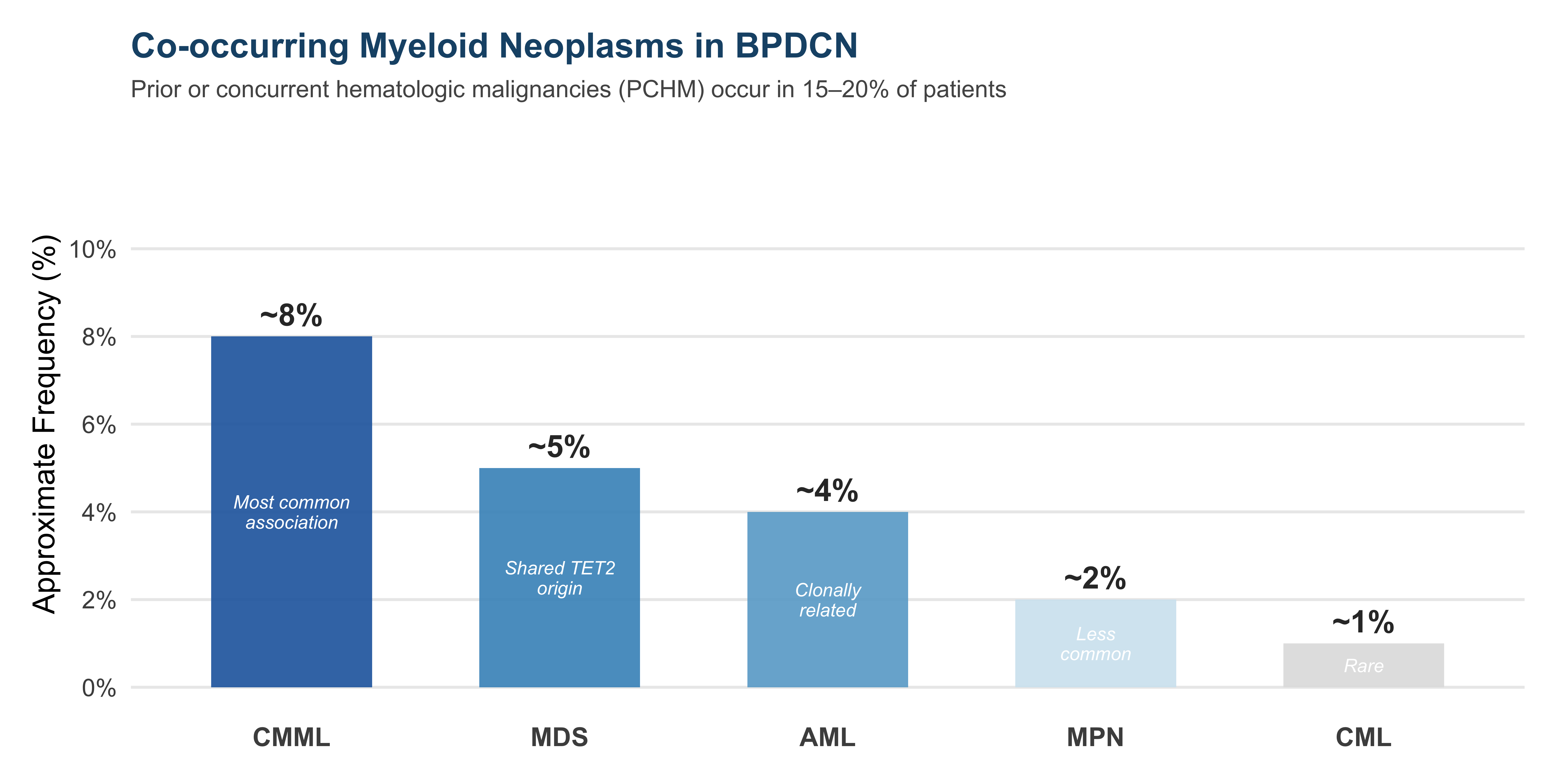
The mutational landscape of BPDCN is complex, with TET2 mutations being the most commonly reported abnormality. Importantly, ~20% of patients have a prior or concurrent hematologic malignancy (PCHM), often sharing a clonal origin with BPDCN.
7.1 Mutational Spectrum
Show code
library(ggplot2)
library(dplyr)

mutations <- tibble(
  Gene = c("TET2", "ASXL1", "ZRSR2", "NRAS", "TP53",
           "IDH2", "SRSF2", "IKZF1", "ETV6", "ARID1A",
           "JAK2", "KRAS", "ATM", "BCOR", "ZEB2"),
  Pathway = c(
    "DNA Methylation", "Chromatin Remodeling", "Splicing", "RAS Signaling", "Tumor Suppressor",
    "DNA Methylation", "Splicing", "Transcription Factor", "Transcription Factor", "Chromatin Remodeling",
    "Cytokine Signaling", "RAS Signaling", "Tumor Suppressor", "Chromatin Remodeling", "Transcription Factor"
  ),
  Frequency = c(55, 30, 25, 20, 18,
                15, 14, 12, 10, 10,
                8, 7, 7, 6, 5)
) |>
  mutate(Gene = factor(Gene, levels = rev(Gene)))

pathway_colors <- c(
  "DNA Methylation" = "#2166ac",
  "Chromatin Remodeling" = "#4393c3",
  "Splicing" = "#67a9cf",
  "Transcription Factor" = "#984ea3",
  "RAS Signaling" = "#d6604d",
  "Cytokine Signaling" = "#f4a582",
  "Tumor Suppressor" = "#e7298a"
)

ggplot(mutations, aes(x = Frequency, y = Gene, fill = Pathway)) +
  geom_col(width = 0.7, alpha = 0.9) +
  geom_text(aes(label = paste0(Frequency, "%")),
            hjust = -0.2, fontface = "bold", size = 3.5, color = "#333333") +
  scale_fill_manual(values = pathway_colors, name = "Functional Pathway") +
  scale_x_continuous(limits = c(0, 70), breaks = seq(0, 60, 10),
                     labels = function(x) paste0(x, "%")) +
  labs(
    title = "BPDCN Mutational Landscape by Functional Pathway",
    subtitle = "TET2 truncating mutations predict worse outcomes | ZRSR2 mutations show sex-biased distribution",
    x = "Approximate Mutation Frequency (%)",
    y = NULL
  ) +
  theme_minimal(base_size = 13) +
  theme(
    plot.title = element_text(face = "bold", size = 16, color = "#1a5276"),
    plot.subtitle = element_text(size = 11, color = "#555555", margin = margin(b = 15)),
    legend.position = "bottom",
    legend.title = element_text(face = "bold"),
    panel.grid.major.y = element_blank(),
    panel.grid.minor = element_blank(),
    axis.text.y = element_text(size = 11, face = "bold"),
    plot.margin = margin(15, 30, 15, 15)
  ) +
  guides(fill = guide_legend(nrow = 2))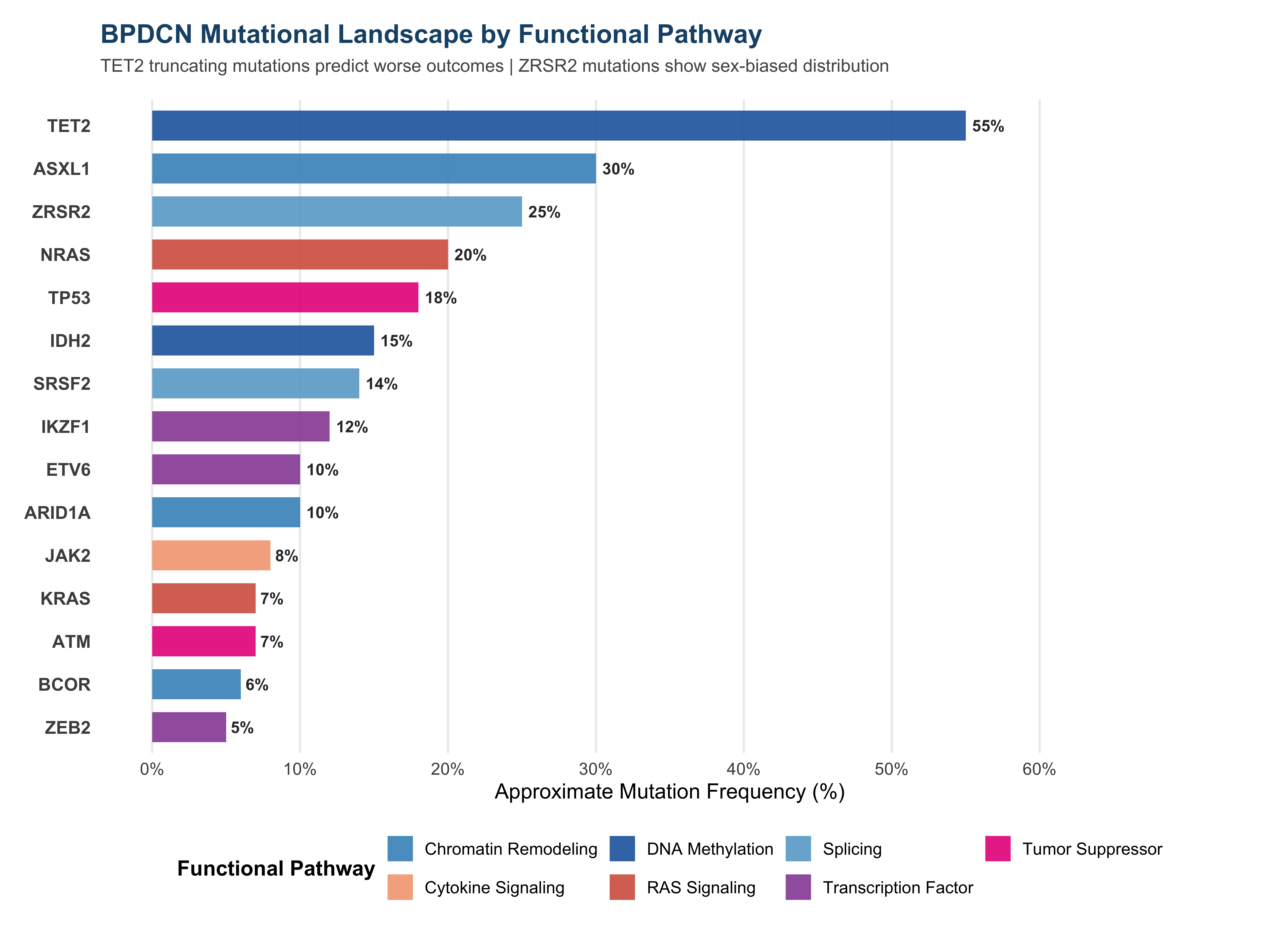
7.2 Genomic Pathway Overview
Show code
import matplotlib.pyplot as plt

categories = [
    'DNA Methylation\n(TET2, IDH2)',
    'Chromatin Remodeling\n(ASXL1, ARID1A, BCOR)',
    'Splicing\n(ZRSR2, SRSF2)',
    'RAS Signaling\n(NRAS, KRAS)',
    'Transcription Factors\n(ETV6, IKZF1, ZEB2)',
    'Tumor Suppressors\n(TP53, ATM)',
    'Cytokine Signaling\n(JAK2, STAT3)'
]
sizes = [35, 20, 15, 12, 10, 5, 3]
colors = ['#2166ac', '#4393c3', '#67a9cf', '#d6604d', '#984ea3', '#e7298a', '#f4a582']
explode = (0.05, 0, 0, 0, 0, 0, 0)

fig, ax = plt.subplots(figsize=(9, 6))
wedges, texts, autotexts = ax.pie(
    sizes, explode=explode, labels=categories, colors=colors,
    autopct='%1.0f%%', startangle=90, pctdistance=0.75,
    textprops={'fontsize': 9}
)

for autotext in autotexts:
    autotext.set_fontweight('bold')
    autotext.set_fontsize(10)
    autotext.set_color('white')

ax.set_title(
    'BPDCN Mutations by Functional Pathway',
    fontsize=16, fontweight='bold', color='#1a5276', pad=20
)

plt.tight_layout()
plt.show()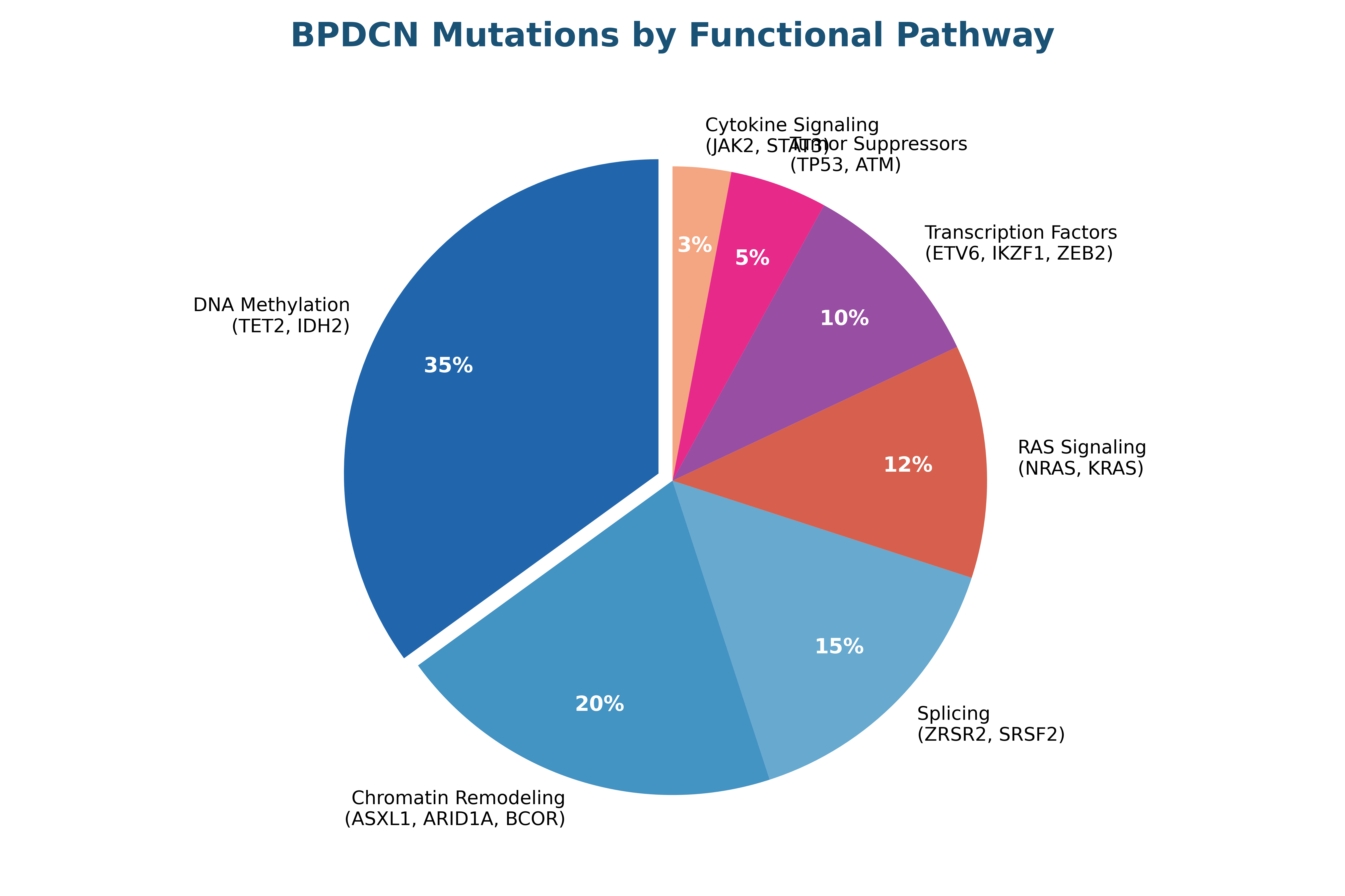
TET2 truncating mutations predict worse outcomes in BPDCN (Beird et al., Blood Adv 2023). ZRSR2 mutations show a sex-biased distribution (located on the X chromosome) and impair plasmacytoid dendritic cell activation and apoptosis (Togami et al., Cancer Discov 2022). Co-occurring myeloid neoplasms (CMML, MDS, AML) are clonally related in at least 10–20% of cases, often sharing a TET2-mutated origin.
8 Staging Workup
Given BPDCN’s propensity for multi-compartment involvement, a comprehensive staging evaluation is essential at diagnosis.
| Evaluation | Modality | Purpose |
|---|---|---|
| Skin assessment | Biopsy + MSWAT scoring | Confirm diagnosis; quantify skin burden |
| Bone marrow | Aspirate + biopsy + flow cytometry | Assess marrow involvement and blast % |
| Peripheral blood | CBC + differential + flow | Detect circulating blasts |
| Imaging | PET-CT | Nodal, visceral, and extranodal disease |
| CSF | Lumbar puncture + cytology + flow | CNS assessment (occult involvement common) |
| Molecular | NGS panel | Identify mutations and co-occurring neoplasms |
| Cytogenetics | Conventional karyotype + FISH | Chromosomal abnormalities (60% have ≥1) |
| Finding | Frequency | Implication |
|---|---|---|
| Occult CNS at diagnosis | ~15% | All patients need LP at diagnosis |
| CNS at any point | Up to 33% | Serial IT prophylaxis recommended |
| CNS at relapse | Common | Highlights need for CNS-penetrant therapy |
| Standard CNS approach | High-risk ALL protocols | IT methotrexate or cytarabine |
| Compartment | Method | Response Criteria |
|---|---|---|
| Skin | Biopsy + MSWAT | Modified from mycosis fungoides/Sézary |
| Bone marrow | IWG AML criteria | Standard morphologic + flow assessment |
| Lymph nodes | Lugano CT criteria | Bidimensional measurements |
| CNS | Serial LP | Cytology + flow clearance |
| Overall | Composite CR | Disappearance in ALL initial disease sites |
9 Co-occurring Myeloid Neoplasms
Show code
library(ggplot2)

pchm_data <- data.frame(
  Condition = factor(c(
    "CMML",
    "MDS",
    "AML",
    "MPN",
    "CML"
  ), levels = c("CMML", "MDS", "AML", "MPN", "CML")),
  Frequency = c(8, 5, 4, 2, 1),
  Note = c(
    "Most common\nassociation",
    "Shared TET2\norigin",
    "Clonally\nrelated",
    "Less\ncommon",
    "Rare"
  )
)

ggplot(pchm_data, aes(x = Condition, y = Frequency)) +
  geom_col(fill = c("#2166ac", "#4393c3", "#67a9cf", "#d1e5f0", "#e0e0e0"),
           width = 0.6, alpha = 0.9) +
  geom_text(aes(label = paste0("~", Frequency, "%")),
            vjust = -0.5, fontface = "bold", size = 5, color = "#333333") +
  geom_text(aes(label = Note, y = Frequency / 2),
            size = 3, color = "white", fontface = "italic", lineheight = 0.9) +
  scale_y_continuous(limits = c(0, 12), breaks = seq(0, 10, 2),
                     labels = function(x) paste0(x, "%")) +
  labs(
    title = "Co-occurring Myeloid Neoplasms in BPDCN",
    subtitle = "Prior or concurrent hematologic malignancies (PCHM) occur in 15–20% of patients",
    x = NULL,
    y = "Approximate Frequency (%)"
  ) +
  theme_minimal(base_size = 14) +
  theme(
    plot.title = element_text(face = "bold", size = 16, color = "#1a5276"),
    plot.subtitle = element_text(size = 11, color = "#555555", margin = margin(b = 15)),
    panel.grid.major.x = element_blank(),
    panel.grid.minor = element_blank(),
    axis.text.x = element_text(size = 12, face = "bold"),
    plot.margin = margin(15, 20, 15, 15)
  )
10 Summary: Diagnostic Checklist
Show code
library(ggplot2)

summary_data <- data.frame(
  Step = factor(c(
    "Clinical suspicion\n(skin + cytopenias)",
    "Tissue biopsy\n(skin or marrow)",
    "Core IHC panel\n(CD123, CD4, CD56)",
    "Extended pDC markers\n(TCF4, TCL1, CD303, CD304)",
    "Lineage exclusion\n(CD3−, CD19−, MPO−, CD14−)",
    "NGS mutational panel",
    "Cytogenetics\n(karyotype + FISH)",
    "PET-CT staging",
    "CSF evaluation\n(LP + flow)",
    "Expert hematopathology\nreview"
  ), levels = rev(c(
    "Clinical suspicion\n(skin + cytopenias)",
    "Tissue biopsy\n(skin or marrow)",
    "Core IHC panel\n(CD123, CD4, CD56)",
    "Extended pDC markers\n(TCF4, TCL1, CD303, CD304)",
    "Lineage exclusion\n(CD3−, CD19−, MPO−, CD14−)",
    "NGS mutational panel",
    "Cytogenetics\n(karyotype + FISH)",
    "PET-CT staging",
    "CSF evaluation\n(LP + flow)",
    "Expert hematopathology\nreview"
  ))),
  Category = c(
    "Clinical", "Pathology", "Immunophenotype", "Immunophenotype",
    "Immunophenotype", "Genomics", "Genomics", "Staging", "Staging", "Final"
  ),
  Priority = c(100, 100, 100, 95, 95, 85, 80, 90, 88, 100),
  bar_val = c(100, 100, 100, 95, 95, 85, 80, 90, 88, 100)
)

cat_colors <- c(
  "Clinical" = "#f4a582",
  "Pathology" = "#d6604d",
  "Immunophenotype" = "#2166ac",
  "Genomics" = "#4daf4a",
  "Staging" = "#4393c3",
  "Final" = "#1a5276"
)

ggplot(summary_data, aes(x = bar_val, y = Step, fill = Category)) +
  geom_col(width = 0.6, alpha = 0.9) +
  scale_fill_manual(values = cat_colors, name = "Diagnostic Domain") +
  scale_x_continuous(limits = c(0, 115)) +
  labs(
    title = "BPDCN Diagnostic Checklist — Essential Elements",
    subtitle = "Comprehensive workup integrating clinical, immunophenotypic, genomic, and staging evaluations",
    x = NULL, y = NULL
  ) +
  theme_void(base_size = 14) +
  theme(
    plot.title = element_text(face = "bold", size = 18, color = "#1a5276",
                              margin = margin(b = 5)),
    plot.subtitle = element_text(size = 12, color = "#555555",
                                 margin = margin(b = 20)),
    axis.text.y = element_text(size = 11, hjust = 1, margin = margin(r = 10)),
    legend.position = "bottom",
    legend.title = element_text(face = "bold", size = 12),
    legend.text = element_text(size = 10),
    plot.margin = margin(20, 50, 20, 20)
  ) +
  guides(fill = guide_legend(nrow = 2))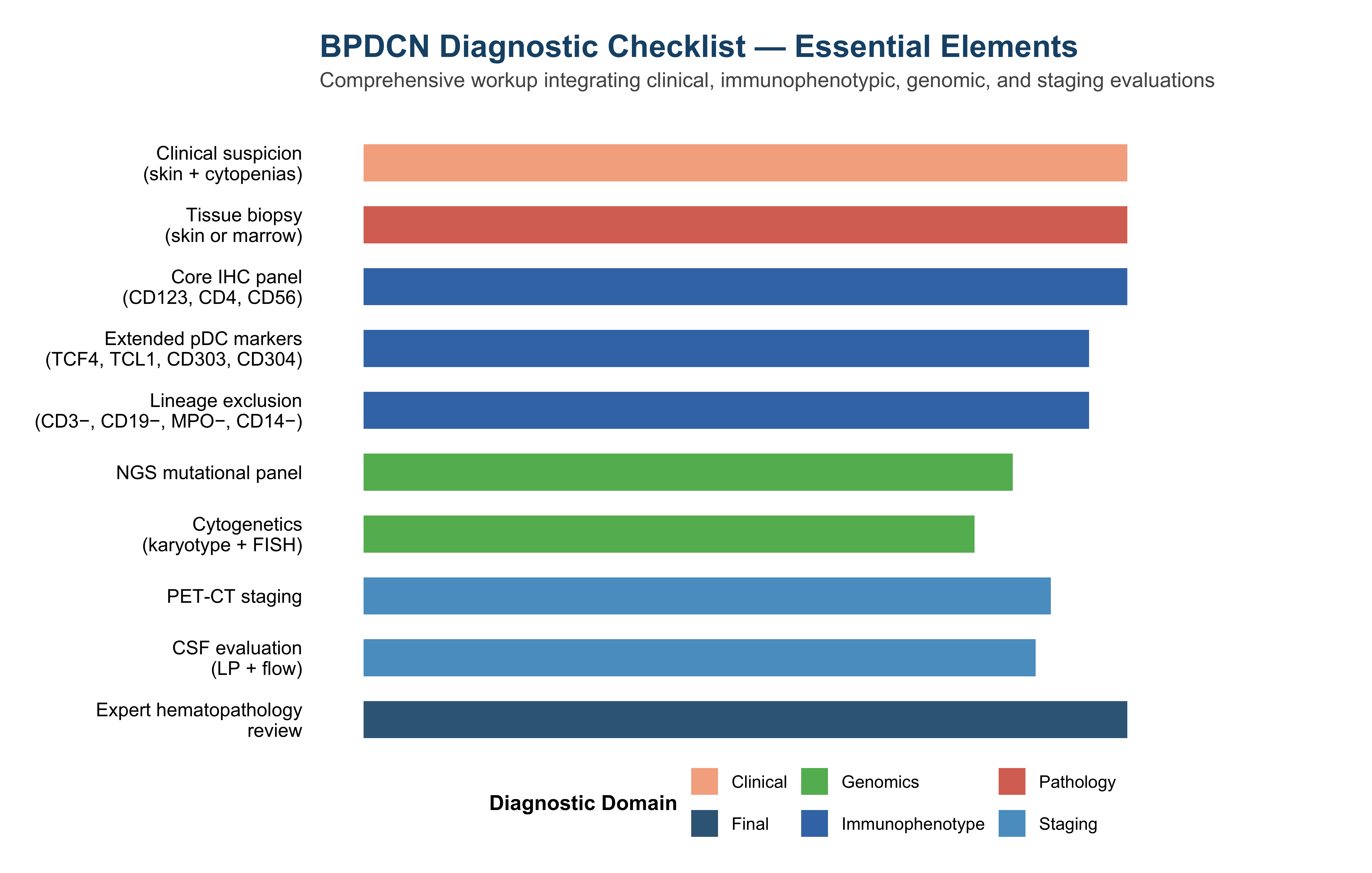
Sources: Kharfan-Dabaja MA, Lane AA, Pemmaraju N. How I treat blastic plasmacytoid dendritic cell neoplasm. Blood. 2025;145(6):567-574. Luskin MR, Lane AA. Tagraxofusp for BPDCN. Haematologica. 2024;109(1):44-52. Pemmaraju N, et al. Pivekimab sunirine in BPDCN. J Clin Oncol. 2026. Pemmaraju N, Lane AA, Sweet KL, et al. Tagraxofusp in BPDCN. N Engl J Med. 2019;380(17):1628-37. Garnache-Ottou F, et al. Blood Adv. 2019;3(24):4238-4251. Togami K, et al. Cancer Discov. 2022;12(2):522-541. Sukswai N, et al. Am J Surg Pathol. 2019;43(10):1429-1437.